

Introduction
Over the past eight blogs, we've built a solid understanding of neural networks. We started with the perceptron, explored multi-layer networks, understood forward propagation, and mastered backpropagation. But there's one more crucial piece of the puzzle we haven't fully explored.
"Neural network ke andar jo 'decision-making' hoti hai, woh activation functions ki wajah se hoti hai."
Activation functions are what give neural networks their power. Without them, a neural network is just a linear regression model. With them, it can learn complex, non-linear patterns.
In this final blog of the ANN series, we'll dive deep into activation functions. We'll understand why we need them, explore all the major types, and learn when to use which one.
Let's begin the final chapter of our ANN journey.
What is an Activation Function?
An activation function is a mathematical function applied to the output of a neuron. It takes the weighted sum z and transforms it into an output a that is passed to the next layer.
z = (w₁ × x₁) + (w₂ × x₂) + ... + (wₙ × xₙ) + b
a = f(z)
Think of it like a gatekeeper. The weighted sum z is like a score. The activation function decides what to do with that score.
"Activation function neuron ka 'decision-maker' hai."
Why Do We Need Activation Functions?
This is the most important question to understand. Let's break it down.
1. Introducing Non-Linearity
Without activation functions, each layer simply performs a linear transformation:
Output = W₂(W₁X + b₁) + b₂ = (W₂W₁)X + (W₂b₁ + b₂)
This is just another linear equation. Multiple linear layers collapse into a single linear layer.
"Activation function ke bina, deep network ek linear model jaisa hai."
With activation functions, we introduce non-linearity:
Output = f₂(W₂ × f₁(W₁X + b₁) + b₂)
This cannot be simplified. The non-linearity allows the network to learn complex patterns.
2. Enabling Deep Learning
Non-linearity allows us to stack layers. Each layer can learn different patterns:
-
Layer 1: Simple edges and corners
-
Layer 2: Shapes and textures
-
Layer 3: Objects and faces
-
Layer 4: Complex concepts
This hierarchy of features is what makes deep learning powerful.
3. Normalizing Output
Activation functions squash the output to a specific range:
-
Sigmoid: (0, 1) = Probability
-
Tanh: (-1, 1) = Zero-centered
-
Softmax: Sums to 1 = Probability distribution
This makes the output interpretable and useful for specific tasks.
4. Enabling Backpropagation
Most activation functions are differentiable. This is crucial for backpropagation. The derivative tells us how to update weights.
5. Biological Plausibility
Activation functions mimic biological neurons, which either fire or don't fire. ReLU, for example, fires for positive inputs and stays silent for negative ones.
Types of Activation Functions
Let's explore each activation function in detail with formulas, graphs, and numerical examples.
1. Step Function (Binary Step)
The simplest activation function of them all.
Formula
f(z) = 1 if z ≥ 0
f(z) = 0 if z < 0
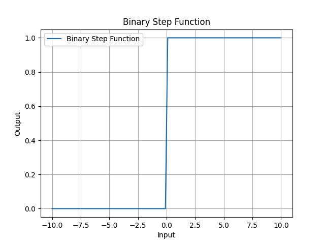
Graph
The step function looks like a staircase. It jumps from 0 to 1 at z = 0.
Advantages
-
Extremely simple
-
Computationally cheap
-
Easy to understand
Disadvantages
-
Not differentiable (derivative is 0 everywhere, undefined at 0)
-
Cannot be used with backpropagation
-
Only works for linearly separable problems
When to Use
-
For understanding fundamental concepts
-
In simple logic gates (AND, OR, NOT)
-
Never in modern deep learning
Numerical Example
Input: z = -2.5
Step Function:
z = -2.5 < 0, so f(z) = 0
Input: z = 3.7
z = 3.7 ≥ 0, so f(z) = 1
Derivative: Not defined (0 everywhere, infinite at z=0)
2. Sigmoid Function
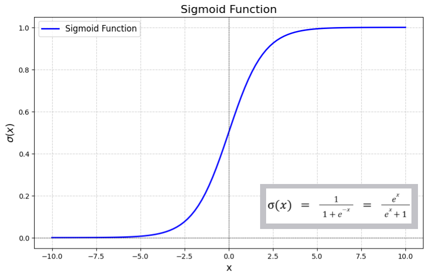
The classic S-shaped curve. One of the most historically important activation functions.
Formula
f(z) = 1 / (1 + e⁻ᶻ)
Graph
The sigmoid produces a smooth S-curve.
Range
(0, 1) — Always positive
Advantages
-
Smooth and differentiable
-
Probabilistic interpretation (output can be treated as probability)
-
Gentle gradients
Disadvantages
-
Vanishing Gradient Problem: For very large or very small z, the gradient approaches 0
-
Non-Zero Centered: Outputs are always positive, causing zigzag updates
-
Computationally expensive (uses exponential)
Derivative
f'(z) = f(z) × (1 - f(z))
This elegant property makes it efficient for backpropagation.
When to Use
-
Output layer of binary classification problems
-
When you need probabilistic outputs
-
Not recommended for hidden layers
Numerical Example
Input: z = 0.5
Sigmoid:
f(0.5) = 1 / (1 + e⁻⁰·⁵)
e⁻⁰·⁵ = 0.6065
f(0.5) = 1 / (1 + 0.6065) = 1 / 1.6065 = 0.6225
Derivative:
f'(0.5) = 0.6225 × (1 - 0.6225)
f'(0.5) = 0.6225 × 0.3775 = 0.2350
Input: z = -2.0
Sigmoid:
f(-2.0) = 1 / (1 + e²)
e² = 7.389
f(-2.0) = 1 / (1 + 7.389) = 1 / 8.389 = 0.1192
Derivative:
f'(-2.0) = 0.1192 × (1 - 0.1192) = 0.1192 × 0.8808 = 0.1049
Notice how the gradient becomes smaller as |z| increases. This is the vanishing gradient problem.
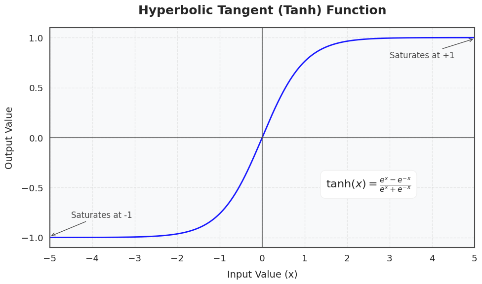
3. Tanh (Hyperbolic Tangent)
The zero-centered cousin of sigmoid.
Formula
f(z) = (eᶻ - e⁻ᶻ) / (eᶻ + e⁻ᶻ)
Alternatively:
f(z) = 2 × sigmoid(2z) - 1
Graph
The tanh is also S-shaped, but ranges from -1 to 1.
Range
(-1, 1) — Zero-centered
Advantages
-
Zero-centered: Leads to faster convergence
-
Stronger gradients than sigmoid
-
Smooth and differentiable
Disadvantages
-
Vanishing Gradient Problem (same as sigmoid)
-
Computationally expensive
Derivative
f'(z) = 1 - f(z)²
When to Use
-
Hidden layers (historically popular)
-
When zero-centered outputs are desired
-
Prefer ReLU in modern architectures
Numerical Example
Input: z = 0.5
Tanh:
tanh(0.5) = (e⁰·⁵ - e⁻⁰·⁵) / (e⁰·⁵ + e⁻⁰·⁵)
e⁰·⁵ = 1.6487, e⁻⁰·⁵ = 0.6065
tanh(0.5) = (1.6487 - 0.6065) / (1.6487 + 0.6065)
tanh(0.5) = 1.0422 / 2.2552 = 0.4621
Derivative:
f'(0.5) = 1 - (0.4621)² = 1 - 0.2135 = 0.7865
Input: z = -2.0
Tanh:
tanh(-2.0) = (e⁻² - e²) / (e⁻² + e²)
e⁻² = 0.1353, e² = 7.389
tanh(-2.0) = (0.1353 - 7.389) / (0.1353 + 7.389)
tanh(-2.0) = -7.2537 / 7.5243 = -0.9640
Derivative:
f'(-2.0) = 1 - (-0.9640)² = 1 - 0.9293 = 0.0707
Notice the gradient is small for large |z|. This is the vanishing gradient problem again.
4. ReLU (Rectified Linear Unit)
The modern workhorse of deep learning. This function changed everything.
Formula
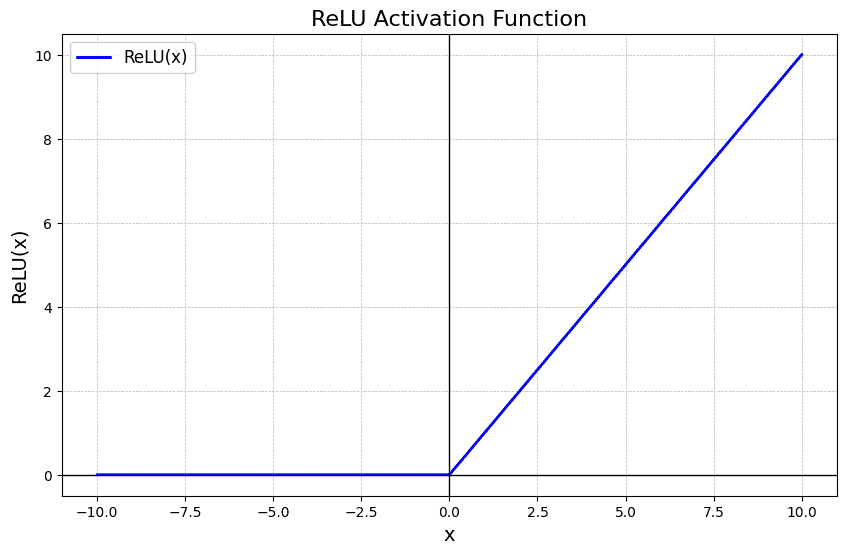
f(z) = max(0, z)
Graph
ReLU is 0 for negative values and linear for positive values.
Range
[0, ∞) — Always non-negative
Advantages
-
Computationally cheap (just max operation)
-
No vanishing gradient (gradient is 1 for z > 0)
-
Sparsity: Many neurons output 0, making the network efficient
-
Enables deep networks
Disadvantages
-
Dying ReLU Problem: Neurons can become permanently inactive
-
Non-zero centered: All outputs are positive
-
Not differentiable at z = 0
Derivative
f'(z) = 1 if z > 0
f'(z) = 0 if z < 0
f'(z) = undefined at z = 0 (can be set to 0 or 1)
When to Use
-
Default choice for hidden layers in modern networks
-
CNNs, deep networks, and most architectures
-
Not recommended for output layers
Numerical Example
Input: z = 0.5
ReLU:
f(0.5) = max(0, 0.5) = 0.5
Derivative:
f'(0.5) = 1 (since z > 0)
Input: z = -2.0
ReLU:
f(-2.0) = max(0, -2.0) = 0
Derivative:
f'(-2.0) = 0 (since z < 0)
Input: z = 0
ReLU:
f(0) = max(0, 0) = 0
Derivative: Undefined (but we set it to 0 in practice)
The Dying ReLU Problem
If a neuron's weighted sum z is always negative, its output is always 0. The gradient is 0, so the neuron never updates. It becomes "dead."
For z < 0: f(z) = 0 and f'(z) = 0
The neuron cannot recover. It is dead forever.
Solutions:
-
Leaky ReLU
-
Parametric ReLU (PReLU)
-
ELU (Exponential Linear Unit)
5. Leaky ReLU
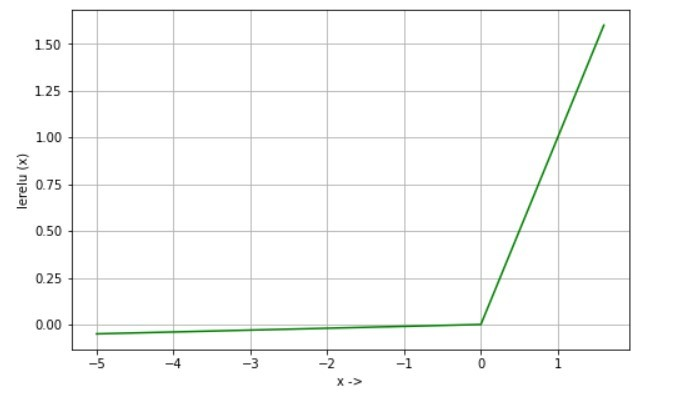
A fix for the dying ReLU problem. Instead of being 0 for negative values, it has a small slope.
Formula
f(z) = z if z ≥ 0
f(z) = αz if z < 0
Where α is a small constant (typically 0.01).
Graph
Leaky ReLU looks like ReLU but with a slight negative slope.
Range
(-∞, ∞) — All real numbers
Advantages
-
No dying ReLU problem (neurons always have some gradient)
-
Same efficiency as ReLU
-
Works in practice
Disadvantages
-
The α parameter must be tuned
-
Not zero-centered
When to Use
-
When ReLU neurons are dying
-
As an alternative to ReLU in hidden layers
Numerical Example
Input: z = 0.5 (α = 0.01)
Leaky ReLU:
f(0.5) = 0.5
Input: z = -2.0
Leaky ReLU:
f(-2.0) = 0.01 × (-2.0) = -0.02
Derivative:
f'(z) = 1 for z > 0
f'(z) = α for z < 0
6. Softmax Function
The special function for multi-class classification.
Formula
f(zᵢ) = eᶻⁱ / Σⱼ eᶻʲ
This converts raw scores into a probability distribution.
Properties
-
Output values sum to 1
-
Each output is between 0 and 1
-
Larger inputs get exponentially larger probabilities
When to Use
-
Output layer of multi-class classification problems
-
When you need a probability distribution
Numerical Example
Input: z = [2.0, 1.0, 0.1]
Softmax:
Step 1: Compute eᶻ for each value
e² = 7.389
e¹ = 2.718
e⁰·¹ = 1.105
Step 2: Sum all values
Sum = 7.389 + 2.718 + 1.105 = 11.212
Step 3: Divide each by the sum
f(z₁) = 7.389 / 11.212 = 0.659
f(z₂) = 2.718 / 11.212 = 0.242
f(z₃) = 1.105 / 11.212 = 0.099
Output: [0.659, 0.242, 0.099]
Check: 0.659 + 0.242 + 0.099 = 1.000 ✓
The first class has the highest probability (0.659).
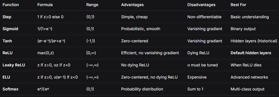
Activation Function Comparison Table
Which Activation Function to Use and When?
This is one of the most common questions in deep learning. Here's a simple guide.
For Hidden Layers
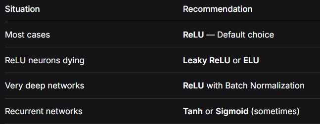
Rule of thumb: "Start with ReLU. Switch only if you have a reason."
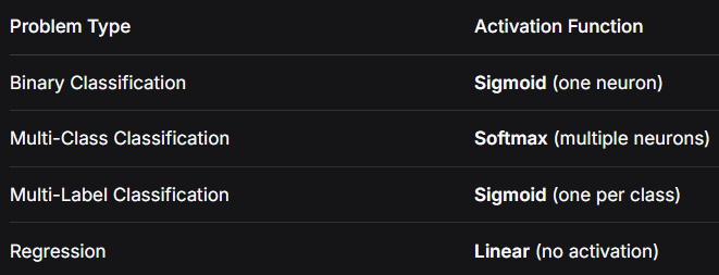
For Output Layers
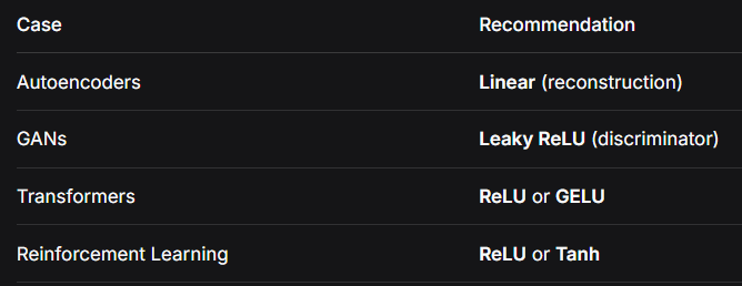
For Special Cases
Why This Matters
Choosing the right activation function can make or break your model.
The ReLU Revolution
Before ReLU, deep networks were hard to train. The vanishing gradient problem made learning slow. ReLU changed everything:
-
Gradient is 1 for z > 0: No vanishing gradient
-
Sparsity: Many neurons are 0, making the network efficient
-
Speed: Just a max operation
This is why ReLU enabled the deep learning revolution.
The Vanishing Gradient Problem
With sigmoid and tanh, gradients become very small for large |z|:
For sigmoid at z = 10: gradient ≈ 0.000045
For sigmoid at z = -10: gradient ≈ 0.000045
In a 10-layer network, multiplying these tiny gradients makes the overall gradient almost 0. The network cannot learn.
ReLU solves this:
For ReLU at z = 10: gradient = 1
For ReLU at z = -10: gradient = 0 (neuron is dead)
This is why ReLU is preferred.
Conclusion
We've reached the end of our ANN series. From the simple perceptron to multi-layer networks, from forward propagation to backpropagation, from activation functions to optimization. We've covered it all.
Activation functions are the heart of neural networks. They make learning possible. They determine what the network can learn. They decide the output format.
Remember these key principles:
Hidden Layers: Use ReLU (or Leaky ReLU if needed)
Binary Output: Use Sigmoid
Multi-Class Output: Use Softmax
Regression: Use Linear (no activation)
Deep Networks: ReLU is your friend
This concludes the ANN series. But our deep learning journey continues. We'll explore more advanced architectures, optimization techniques, and real-world applications.
"ANN ki kahani yahan khatam hoti hai, lekin deep learning ki kahani abhi shuru hui hai."
Thank you for being on this journey with me. See you in the next series!